Lab on Dynamic Discrete Choice
28 February, 2023
- Consider a simple saving problem (cake eating)
- Explain Bellman problem without uncertainty
- Explain Bellman problem with uncertainty
- Solve simple consumption saving problem
- Simulate transitory and permanent policies
- Plot a fit using some simple distance, an indirect inference estimator
We consider here discrete choices over a set of alernatives. The utility of the agent is modeled as
Cake eating
Imagine you a given a cake os size \(S\), and you need to decide how much to eat everyday. How would you formulate the problem?
\[ \max_{c_t} \sum_{t=0}^\infty \beta^t u( c_t) \quad s.t. \quad \sum_{t=0}^\infty c_t \leq S\] One can write the Lagrangian of this problem and find:
\[L = \sum_{t=0}^\infty \beta^t u( c_t) - \lambda \Big( \sum_{t=0}^\infty c_t - S \Big)\]
This gives the following FOCs:
\[ \beta^t u'(c_t) = \lambda \]
Consider a CRRA utility function \(u(c)=\frac{c^{1-\gamma}}{1-\gamma}\) which gives \(u'(c)=c^{-\gamma}\) and hence \[ \sum_{t=0}^\infty c_t = \sum_{t=0}^\infty \Big( \frac{\lambda}{\beta^t} \Big)^{-\frac{1}{\gamma} } = \frac{\lambda^{-\frac{1}{\gamma}}}{1-\beta^{1/\gamma-1}} =S \] hence we get that the consumption will be
\[c_t = \Big( \frac{\lambda}{\beta^t} \Big)^{-\frac{1}{\gamma} } = (1-\beta^{1/\gamma-1})\beta^{t/\gamma}S\]
As an exercise, one can plot this for different values of \(\beta\) and \(\gamma\).
library(data.table)
library(ggplot2)
set.seed(4325342)
A recursive formulation
Let’s introduce \(V(S)\) as the present value, the life time value of having a cake of size \(S\) today and consuming optimally in the future.
\[V(S) = \max_{c_t} \sum_{t=0}^\infty \beta^t u( c_t) \quad s.t. \quad \sum_{t=0}^\infty c_t \leq S\] A simple derivation establishes that:
\[V(S) = \max_{c} u(c) + \beta V(S-c) \]
The bus engine problem
Imagine that we want to model the decision to replace the engine on in a fleet of buses. This is the premise of a seminal paper by John Rust Optimal Replacement of GMC Bus Engines: An Empirical Model of Harold Zurcher. Here is a simple version of it:
- the state is \(x_t\), the mileage of the engine
- every period, the bus delivers profit as a function of \(x_t\), call it \(p(x_t)\)
- the bus owner Mr Zurcher, can decide to replace the engine at cost \(C\) in which case \(x_t\) goes back to \(0\)
- the bus dies with probability a function of \(x_t\) in which case the owner gets \(0\)
- the owner discounts at rate \(\beta\)
- every period, the bus accumulates a \(u\) miles
Using our Bellman tool we can write the optimal decision for this problem recursively:
\[ V(x) = \max \{ p(x) + \lambda(x)\beta V(x+u) , -C + \beta V(0) \} \] We can see that this will have a threshold property. In practice the decision won’t be as clear as a simple threshold. We want to allow for some randomness. We then add a logit preference shock \(\xi\) to the different between the two options. We then remember that we can transform the max into a log-sum-exp.
\[ V(x) = \log\Big( \exp \Big[p(x) + \lambda(x)\beta V(x+u)\Big] + \exp \Big[ -C + \beta V(0) \Big] \Big) + \gamma \]
There is not hope to solve this problem in closed form. We tackle it numerically.
n      = 100 # number of grid point for V
V      = rep(0,n)
x      = seq(0,100,l=n)
lambda = 1/(1+exp(0.1*(x-50))) # break probability
beta   = 0.9
C      = 2
P      = exp(-0.01*x) # profit function
In = c(2:n,n)         # increasing x by 1

# Solving the Bellman equation using a fix point approach
rr = data.frame()
for (i in 1:300) {
  rr = rbind(rr,data.frame(x=x,V=V,rep=i,v1=P + lambda*beta*V[In],v2=-C + beta*V[1] ))
  V2 = log( exp( P + lambda*beta*V[In]) +  exp(-C + beta*V[1] )  ) + 0.56
  dist = mean((V2-V)^2)
  V=V2
}

# plotting different iterations
rr = data.table(rr)
ggplot(rr[rep<100],aes(x=x,y=V,group=rep,color=factor(rep))) +
  geom_line() + ggtitle("Belman iteration for V") + theme_bw() + theme(legend.position="none")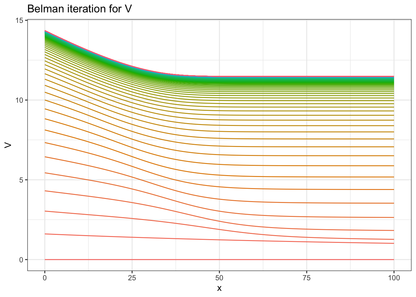
# plotting each options
ggplot(rr[rep %in% c(5,10,60)],aes(x=x,y=v1,group=rep,color=factor(rep))) +
  geom_line(linetype=2) +
  geom_line(aes(y=V)) +
  geom_hline(aes(yintercept =v2,color=factor(rep)) ,linetype=2) +
  theme_bw() +
  ggtitle("plotting value of replacing versus not")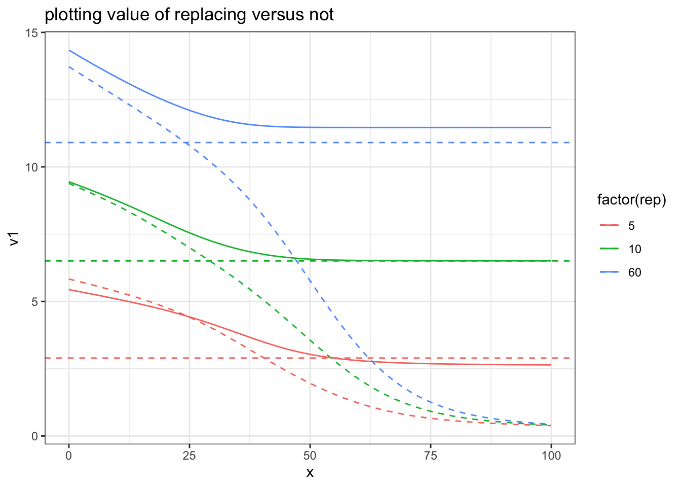
# we can look at the probability to replace
rr2 = data.frame(x=x, V=V, rep=i, v1=P + lambda*beta*V[In], v2=-C + beta*V[1] )
ggplot(rr2,aes(x=x,y=1/(1+exp(v1-v2)))) + geom_line() +
  theme_bw() +
  ggtitle("Probability of replacing")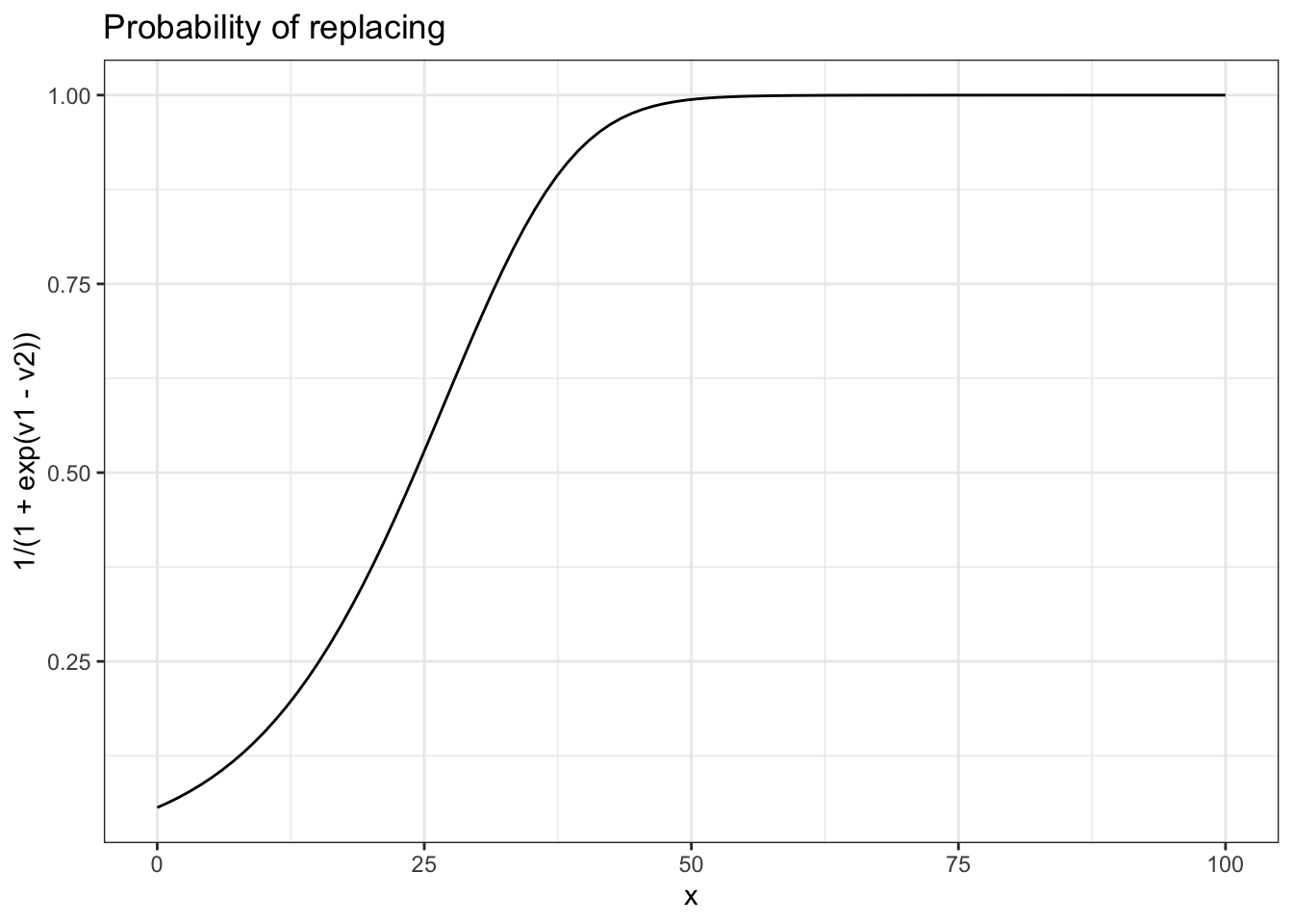
# final value
ggplot(rr2,aes(x=x,y=V)) + geom_line() +
  theme_bw() +
  ggtitle("Value function")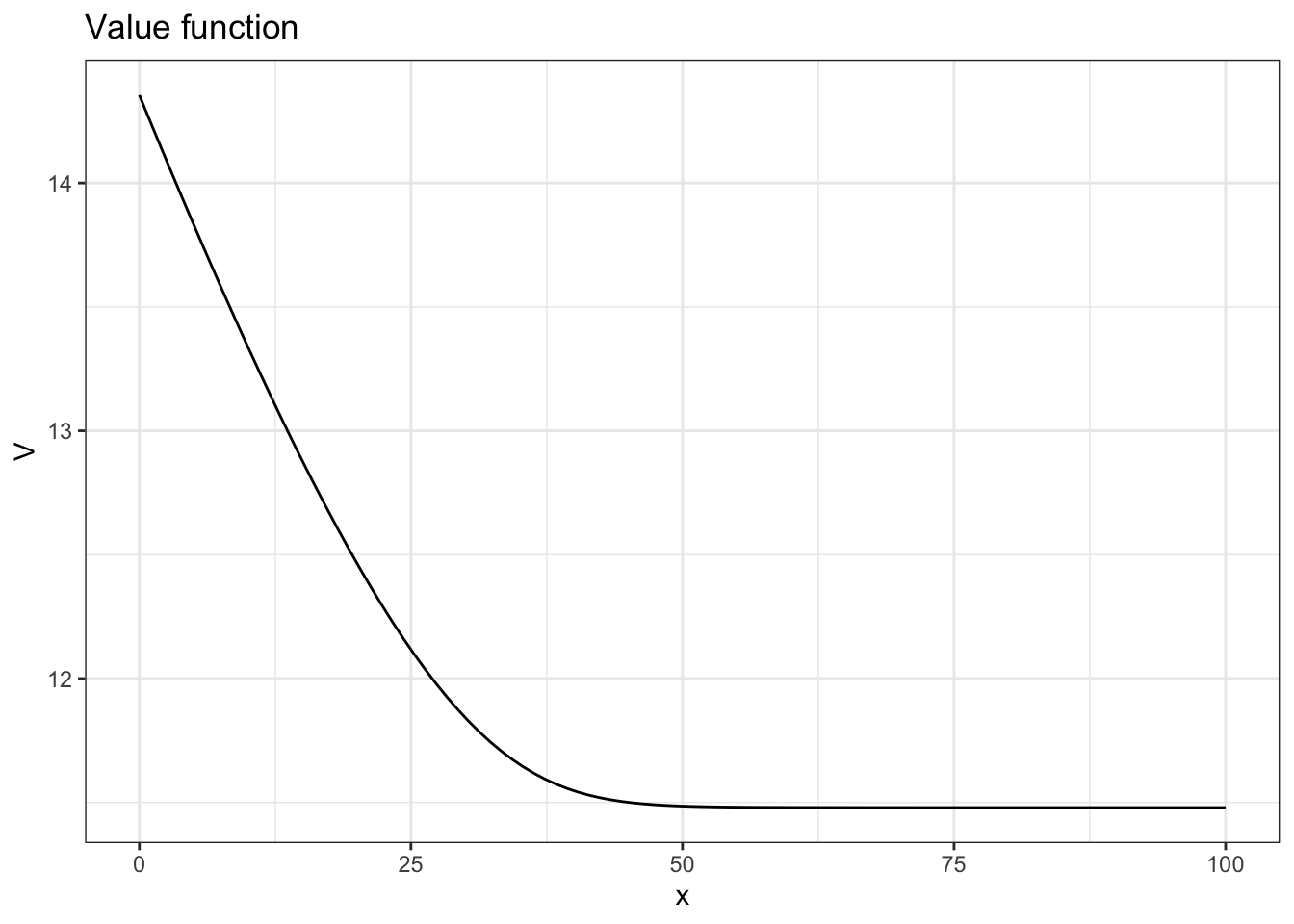
simulating data
We simulate a fleet of 100 buses, each over 100 periods.
PR1 = 1/(1+exp( P + lambda*beta*V[In] - (-C + beta*V[1])))

rr = data.frame()
for (i in 1:100) {
  rrr = data.frame()
  x=1
  l=1
  R=0
  for (t in 1:100) {

    if (l==0) {
      rrr = rbind(rrr,data.frame(i=i,t=t,x=0,l=0,profit=0,R=0))
      next
    }

    # draw the maintenance choice
    if (PR1[x]>runif(1)) {
      R=1
      profit = -C

    } else {
      R=0
      profit = P[x]

      if (lambda[x]<runif(1)) {
        l=0
      }
    }
    rrr = rbind(rrr,data.frame(i=i,t=t,x=x,l=1,profit=profit,R=R))
    if (R==1) {
       x=1
    } else {
      x= x+1
    }
  }
  rr = rbind(rr,rrr)
}

data = data.table(rr)
data[,sum(l==1),i][,mean(V1)]
## [1] 68.72ggplot(data[i==5],aes(x=t,y=profit)) + geom_line() + theme_bw()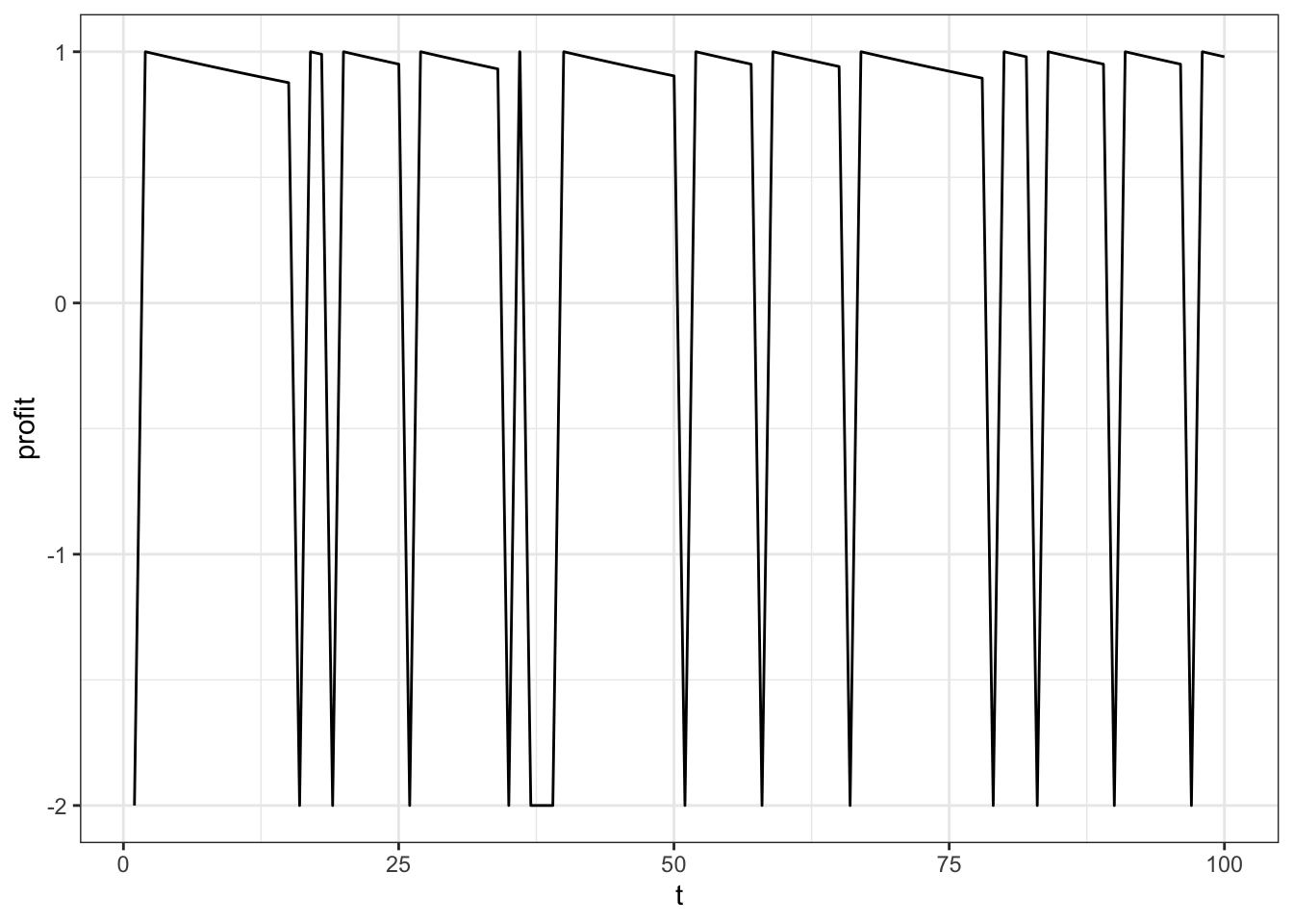
ggplot(data[i==1],aes(x=t,y=x)) + geom_line() + theme_bw()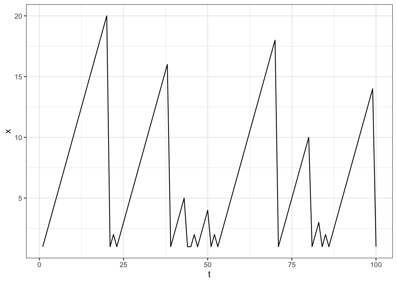
We take a look at the raw data
data## i t x l profit R
## 1: 1 1 1 1 1.0000000 0
## 2: 1 2 2 1 0.9899498 0
## 3: 1 3 3 1 0.9800007 0
## 4: 1 4 4 1 0.9701515 0
## 5: 1 5 5 1 0.9604013 0
## ---
## 9996: 100 96 0 0 0.0000000 0
## 9997: 100 97 0 0 0.0000000 0
## 9998: 100 98 0 0 0.0000000 0
## 9999: 100 99 0 0 0.0000000 0
## 10000: 100 100 0 0 0.0000000 0Eventually all buses die, we can plot the survival probability:
plot( data[, mean(R), by=t]$V1)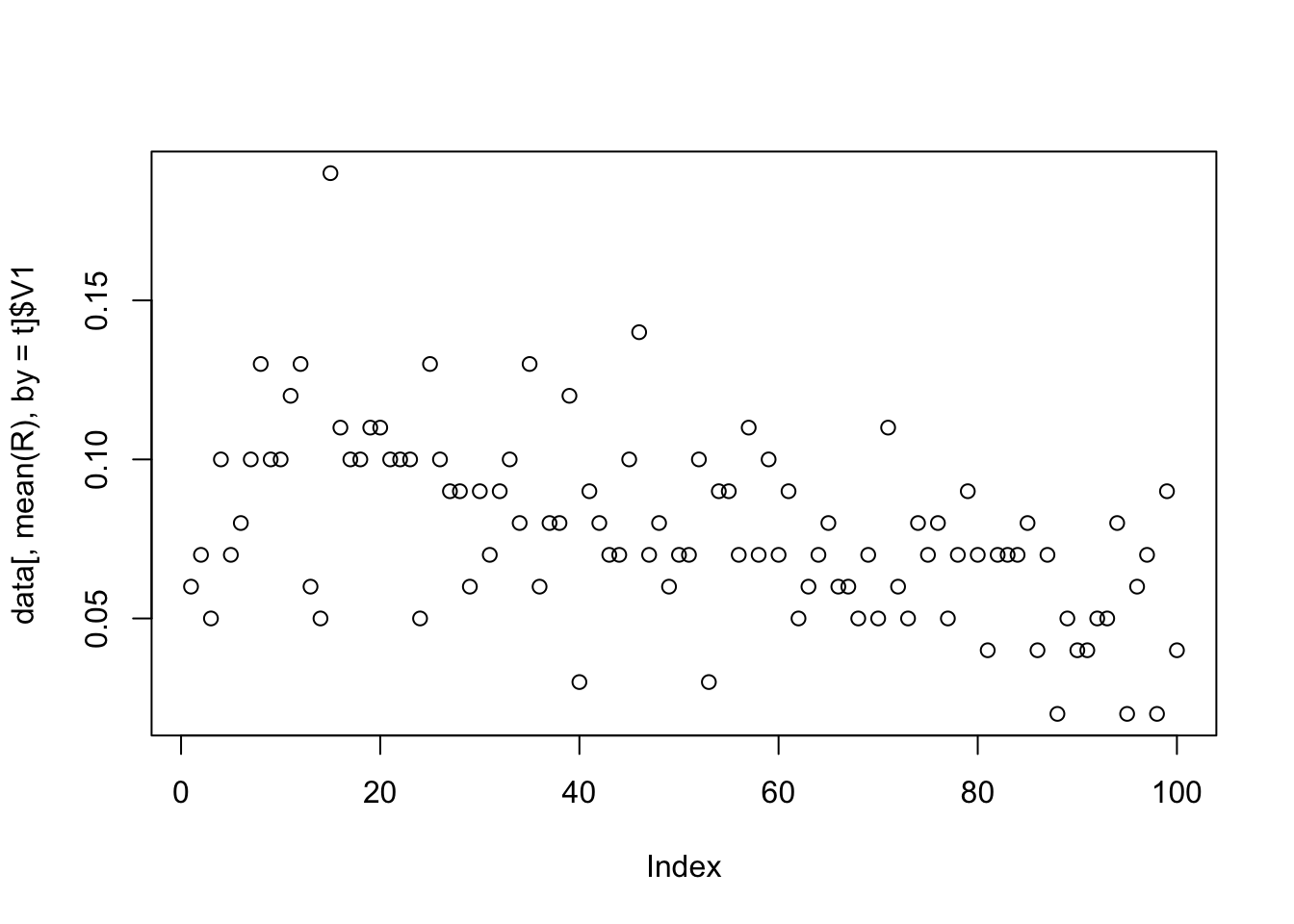
Writing a likelihood
We can write the likelihood of the decision and miles and sum across individuals
lik <- function(theta) {
  n      = 100
  V      = rep(0,n)
  x      = seq(0,100,l=n)
  lambda = 1/(1+exp(0.1*(x-50)))
  beta   = 0.9
  C      = theta
  P      = exp(-0.01*x)
  In = c(2:n,n)

  rr = data.frame()
  for (i in 1:100) {
    rr = rbind(rr,data.frame(x=x,V=V,rep=i,v1=P + lambda*beta*V[In],v2=-C + beta*V[1] ))
    V2 = log( exp( P + lambda*beta*V[In]) +  exp(-C + beta*V[1] )  ) + 0.56
    dist = mean((V2-V)^2)
    V=V2
  }
  Pr  =1/(1+exp( P + lambda*beta*V[In] - (-C + beta*V[1])))
  data[l==1,sum(log(Pr[x])*(R==1) + log(1-Pr[x])*(R==0)) ]
}


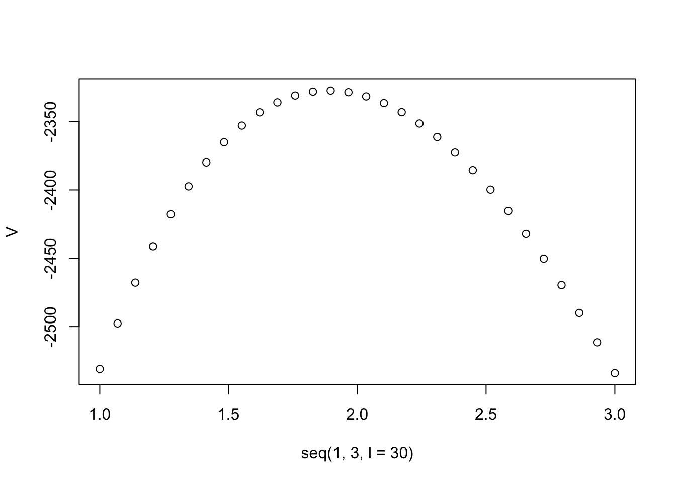
V = sapply(seq(1,3,l=30),lik)
plot(seq(1,3,l=30),V)