ECON 21130 - R tutorial
Wooyong Lee
Basics
value assignment
Some languages like C requires to specify the type of the variable
first and then assign numbers, e.g. int abc; abc = 2;. But
R does not require such thing. R automatically generates the variable
and changes the variable type accordingly.
# the basic value assignment operator that always works
abc <- 2 # in this line, R creates the variable "abc" and assigns 2
abc
## [1] 2# the easy-to-use operator that rarely, but not never, produces error
abc = 2
abc## [1] 2# you can also assign arrays
abc = c(1,2,3,4,5)
abc## [1] 1 2 3 4 5# assigning the integer sequence
abc = 1:5
abc## [1] 1 2 3 4 5abc = 3:(-2)
abc## [1] 3 2 1 0 -1 -2# you can use the function "rep" to create repeating vectors
abc = rep(2, 5)
abc## [1] 2 2 2 2 2abc = rep(c(1,2,3), 5)
abc## [1] 1 2 3 1 2 3 1 2 3 1 2 3 1 2 3# you can use the function "seq" to assign an equispaced sequence
abc = seq(from=0, to=1, by=0.1)
abc## [1] 0.0 0.1 0.2 0.3 0.4 0.5 0.6 0.7 0.8 0.9 1.0abc = seq(from=0, to=1, length=11)
abc## [1] 0.0 0.1 0.2 0.3 0.4 0.5 0.6 0.7 0.8 0.9 1.0writing functions
You can write the custom functions in R easily. The functions do not need to be written in separate files while some languages like Matlab requires to do so.
# to write a custom function, assign FUNCTION to a VARIABLE
add = function(x,y) {
  return(x+y)
}
square = function(x) {
  return(x^2)
}

# the return statement can be omitted. R returns what is written in the last line.
square_noReturnStatement = function(x) {
  x^2
}

# to call a function, write the name and put arguments inside the bracket
abc = 3
add(x=abc, y=2)
## [1] 5square(x=3)## [1] 9square_noReturnStatement(x=3)## [1] 9# you can omit the labels
add(abc,2)## [1] 5# of course you can assign the returned value to a variable
result = square(abc)
result## [1] 9By the way, now we can have better understanding of what we mean by R automatically changing the variable types:
# right now, a function is assigned in the variable "add":
add
## function(x,y) {
## return(x+y)
## }
## <bytecode: 0x134c37d80># we know it works as a function
add(abc, 2)## [1] 5# let's assign a number to "add":
add = 3;
add## [1] 3# then the variable "add" is no longer a function:
add(abc, 2)## Error in add(abc, 2): could not find function "add"local and parent environment
Consider the following code.
myFunc = function(x) {
  xSquare = x^2
  return(xSquare/3)
}

myFunc(x = 2)
## [1] 1.333333xSquare## Error in eval(expr, envir, enclos): object 'xSquare' not foundWe see that xSquare is not defined, even though it
should have been used in myFunc. What happens in R, and in
many other programming languages, is the following. When we call
myFunc, R creates a sub-environment (i.e. a storage space)
and define xSquare there. Then, when it returns
xSquare/3 and escape myFunc, it deletes the
sub-environment. Therefore, xSquare is not stored
anymore.
The sub-environment is like a child of the original environment, and so we call the original one as the parent environment in the perspective of sub-environment. The very top environment is called the global environment.
We call the variables in the current environment as “local variables”.
Now consider the following code.
myFunc = function(x) {
  xSquare = x^2
  return(xSquare/3)
}

myFunc2 = function(x) {
  xInverse = 1/x
  resultMyFunc = myFunc(xInverse)
  return(resultMyFunc)
}

myFunc3 = function(x) {
  xCube = x^3
  resultMyFunc2 = myFunc2(xCube)
  return(resultMyFunc2)
}

myFunc3(x = 2)
## [1] 0.005208333When we call myFunc3 in the last line, R creates a
sub-environment for myFunc3. Then, when
myFunc3 calls myFunc2 within its code, R
creates an environment for myFunc2 that is a
sub-environment of myFunc3. Similarly, when
myFunc2 calls myFunc, R creates another
sub-environment.
When the function creates the sub-environment, it stores the
arguments of the function in the environment. In the above example,
every environment has x variable, although they will all
have different values.
How much the sub-environment can access variables in the parent environment is different across languages. In R, the functions can read and change values of the variables in the parent environments.
myFuncValue = 0

myFunc5 = function() {

  print(myFuncValue)
  myFuncValue = 2

  myFunc4 = function() {

    print(myFuncValue)
    myFuncValue = 1
    print(myFuncValue)
  }

  myFunc4()
  print(myFuncValue)
}

myFunc5()
## [1] 0
## [1] 2
## [1] 1
## [1] 2print(myFuncValue)## [1] 0In the above code, myFuncValue is present in all of the
environments. The function always first search for the local variable
when it needs to access the variable.
Now let’s see what happens if we define myFunc4 not in
the environment of myFunc5 but in the global
environment.
myFuncValue = 0

myFunc4 = function() {

  print(myFuncValue)
  myFuncValue = 1
  print(myFuncValue)
}

myFunc5 = function() {

  print(myFuncValue)
  myFuncValue = 2

  myFunc4()
  print(myFuncValue)
}

myFunc5()
## [1] 0
## [1] 0
## [1] 1
## [1] 2print(myFuncValue)## [1] 0In R, we can also change the value of the variable in the parent
environment using <<-.
# let's add lines that orders the functions to print variables of parent environments:

xx = 2

myFunc6 = function(x) {
  xSquare = x^2
  myFunc7()
  return(xSquare)
}

myFunc7 = function() {
  xx <<- 0
}

myFunc6(x = xx)
## [1] 4xx## [1] 0However, accessing variables of the parent environment is not recommended, as it is very likely to produce errors and wrong results. If you need to access variables of the parent environment, always pass it to sub-environment by putting them as arguments.
a = 2
b = 3

myFunc8 = function(x) { # not recommended!
  return(x + a + b)
}

myFunc9 = function(x,a,b) {
  return(x + a + b) # as mentioned before, the function will use the "local" a and b.
}
matrix, array and data.frame
There may be other ways, but one way to create a matrix is the following.
mat = matrix(0, nrow=3, ncol=2)
mat
## [,1] [,2]
## [1,] 0 0
## [2,] 0 0
## [3,] 0 0sampleArray = c(1,2,3,4,5,6)
mat = matrix(sampleArray, nrow=3, ncol=2)
mat## [,1] [,2]
## [1,] 1 4
## [2,] 2 5
## [3,] 3 6mat = matrix(sampleArray, nrow=3, ncol=2, byrow = TRUE)
mat## [,1] [,2]
## [1,] 1 2
## [2,] 3 4
## [3,] 5 6# you can access the entries in a usual way.
# In some languages such as C, the first entry is labeled 0.
# In R, the first entry is 1.
mat[1,1]## [1] 1mat[3,2]## [1] 6mat[0,1]## numeric(0)# you can also access rows or columns
mat[3,]## [1] 5 6mat[,2]## [1] 2 4 6# you can also call the submatrices
mat[c(1,2),]## [,1] [,2]
## [1,] 1 2
## [2,] 3 4# a useful trick
mat[c(1,3,3,3,2,1,3),]## [,1] [,2]
## [1,] 1 2
## [2,] 5 6
## [3,] 5 6
## [4,] 5 6
## [5,] 3 4
## [6,] 1 2
## [7,] 5 6The array function with 2 dimensions also returns a
matrix. It is also useful in producing 3 dimensional arrays.
arr = array(0, dim = c(3,2))
arr## [,1] [,2]
## [1,] 0 0
## [2,] 0 0
## [3,] 0 0arr = array(0, dim = c(3,2,4))
arr## , , 1
##
##      [,1] [,2]
## [1,]    0    0
## [2,]    0    0
## [3,]    0    0
##
## , , 2
##
##      [,1] [,2]
## [1,]    0    0
## [2,]    0    0
## [3,]    0    0
##
## , , 3
##
## [,1] [,2]
## [1,] 0 0
## [2,] 0 0
## [3,] 0 0
##
## , , 4
##
## [,1] [,2]
## [1,] 0 0
## [2,] 0 0
## [3,] 0 0The data.frame is a variable type that handles the
datasets.
ctrs = c("U.S.", "Canada", "Mexico")
pops = c(318.9, 35.16, 122.3)

# you create a data frame as follows:
df = data.frame(Country=ctrs, Population=pops)
df
## Country Population
## 1 U.S. 318.90
## 2 Canada 35.16
## 3 Mexico 122.30The data.frame is a matrix with the data manipulation
capabilities.
# you can access the entries like the matrix
df[3,2]
## [1] 122.3# you can also access a column by its name. Use money symbol.
df$Population## [1] 318.90 35.16 122.30# you can also subset the dataset
subDF = subset(df, Population >= 100)
subDF## Country Population
## 1 U.S. 318.9
## 3 Mexico 122.3subDF = subset(df, Population >= 100, select = c("Country"))
subDF## Country
## 1 U.S.
## 3 Mexicodata.table
We may use data.table intead of data.frame
in the class. It is an enhancement of data.frame which is
created by contributors of R community.
data.table is not automatically installed with base R.
We need to install a “package” for data.table, which is
basically a collection of codes. We install the package in our computer
by the following code. R uses internet and downloads the package from
the R package database.
# the name of the package that allows us to use data.table is "data.table".
install.packages("data.table")
Now we have installed the package. As we do when we install and use computer programs like MS Office, We need to “execute” or “load” the package to use it. We load the package by the following code:
library(data.table)Now we discuss how data.frame works. It works like
data.frame.
# recall:
ctrs
## [1] "U.S." "Canada" "Mexico"pops## [1] 318.90 35.16 122.30# create datatable
dt = data.table(Country=ctrs, Population=pops)
dt## Country Population
## 1: U.S. 318.90
## 2: Canada 35.16
## 3: Mexico 122.30We can also transform data.frame into data.table.
# recall:
df
## Country Population
## 1 U.S. 318.90
## 2 Canada 35.16
## 3 Mexico 122.30class(df)## [1] "data.frame"# transform.
dt = as.data.table(df)
dt## Country Population
## 1: U.S. 318.90
## 2: Canada 35.16
## 3: Mexico 122.30class(dt)## [1] "data.table" "data.frame"data.table has additional features compared to
data.frame. For example, to subset a data.table, do the
following.
# subset rows with pop >= 100
dt[Population >= 100]
## Country Population
## 1: U.S. 318.9
## 2: Mexico 122.3# subset rows but choose the country column only.
dt[Population >= 100, Country]## [1] "U.S." "Mexico"# if you want to be still in the data.table format:
dt[Population >= 100, list(Country)]## Country
## 1: U.S.
## 2: Mexicoclass(dt[Population >= 100, list(Country)])## [1] "data.table" "data.frame"We will see other features of data.table soon. For more
information, look at https://github.com/Rdatatable/data.table/wiki/Getting-started,
which is a webpage created by the author of data.table
package.
list
list is a variable type that can store various
sub-variables. It is like struct in C.
abc = list(a=3, b="John Doe", c=123.456)

# to access the sub-variables, call them using the money symbol:
abc$a
## [1] 3abc$b## [1] "John Doe"abc$c## [1] 123.456Inside the list, you can save everything as a
sub-variable. You can save functions, you can save matrices, you can
save a list inside a list, and so on. The following example stores
various model primitives of a matching model in Labor economics.
# model primitives
model = list(
  r = 0.05, # interest rate
  s = 0.02, # separation rate
  matchFunc = function(u,v) { 0.4 * u^0.5 * v^0.5 }, # matching function
  b = 0, # unemployment benefit
  c = 0, # cost of vacancy
  alpha = 0.5, # bargaining power
  prodFunc = function(x,y) { (x^(-2) + y^(-2))^(1/(-2)) + 0.2 } # production function
)
We can call a function inside the list in a usual way:
model$prodFunc(1,2)## [1] 1.094427Instead of assigning names to the sub-variables, we can leave the names blank, in which case the serial numbers are assigned.
abc = list(3, "John Doe", 123.456)
abc
## [[1]]
## [1] 3
##
## [[2]]
## [1] "John Doe"
##
## [[3]]
## [1] 123.456# to access the elements of the list, use the double brackets:
abc[[1]]## [1] 3abc[[2]]## [1] "John Doe"abc[[3]]## [1] 123.456syntax
If you are familiar with syntax of other languages such as matlab,
stata, python, etc., the syntax is very much similar in R. For example,
the for loop looks like this:
# the canonical for loop with natural numbers
sum = 0
for(i in 1:4) {
  sum = sum + i
}
sum
## [1] 10# the loop works for ANY array
greekLetterArray = c("Alpha", "Beta", "Gamma", "Delta")
for(greekLetter in greekLetterArray) {
print(greekLetter)
}## [1] "Alpha"
## [1] "Beta"
## [1] "Gamma"
## [1] "Delta"I will not spend time on the syntax, but you can use google to learn how to write a certain syntax, or you can come to the office hour.
The plyr package
The plyr package is a package for data manipulation.
Let’s look at how the functions in the plyr package are
used by example. First, let’s take a dataset from the MASS
package. The MASS package is pre-installed in R, and so we
can simply load it without installing it.
library(MASS)

# the MASS package contains a dataset named "Insurance" which is a dataset about the insurance claims.
Insurance
## District Group Age Holders Claims
## 1 1 <1l <25 197 38
## 2 1 <1l 25-29 264 35
## 3 1 <1l 30-35 246 20
## 4 1 <1l >35 1680 156
## 5 1 1-1.5l <25 284 63
## 6 1 1-1.5l 25-29 536 84
## 7 1 1-1.5l 30-35 696 89
## 8 1 1-1.5l >35 3582 400
## 9 1 1.5-2l <25 133 19
## 10 1 1.5-2l 25-29 286 52
## 11 1 1.5-2l 30-35 355 74
## 12 1 1.5-2l >35 1640 233
## 13 1 >2l <25 24 4
## 14 1 >2l 25-29 71 18
## 15 1 >2l 30-35 99 19
## 16 1 >2l >35 452 77
## 17 2 <1l <25 85 22
## 18 2 <1l 25-29 139 19
## 19 2 <1l 30-35 151 22
## 20 2 <1l >35 931 87
## 21 2 1-1.5l <25 149 25
## 22 2 1-1.5l 25-29 313 51
## 23 2 1-1.5l 30-35 419 49
## 24 2 1-1.5l >35 2443 290
## 25 2 1.5-2l <25 66 14
## 26 2 1.5-2l 25-29 175 46
## 27 2 1.5-2l 30-35 221 39
## 28 2 1.5-2l >35 1110 143
## 29 2 >2l <25 9 4
## 30 2 >2l 25-29 48 15
## 31 2 >2l 30-35 72 12
## 32 2 >2l >35 322 53
## 33 3 <1l <25 35 5
## 34 3 <1l 25-29 73 11
## 35 3 <1l 30-35 89 10
## 36 3 <1l >35 648 67
## 37 3 1-1.5l <25 53 10
## 38 3 1-1.5l 25-29 155 24
## 39 3 1-1.5l 30-35 240 37
## 40 3 1-1.5l >35 1635 187
## 41 3 1.5-2l <25 24 8
## 42 3 1.5-2l 25-29 78 19
## 43 3 1.5-2l 30-35 121 24
## 44 3 1.5-2l >35 692 101
## 45 3 >2l <25 7 3
## 46 3 >2l 25-29 29 2
## 47 3 >2l 30-35 43 8
## 48 3 >2l >35 245 37
## 49 4 <1l <25 20 2
## 50 4 <1l 25-29 33 5
## 51 4 <1l 30-35 40 4
## 52 4 <1l >35 316 36
## 53 4 1-1.5l <25 31 7
## 54 4 1-1.5l 25-29 81 10
## 55 4 1-1.5l 30-35 122 22
## 56 4 1-1.5l >35 724 102
## 57 4 1.5-2l <25 18 5
## 58 4 1.5-2l 25-29 39 7
## 59 4 1.5-2l 30-35 68 16
## 60 4 1.5-2l >35 344 63
## 61 4 >2l <25 3 0
## 62 4 >2l 25-29 16 6
## 63 4 >2l 30-35 25 8
## 64 4 >2l >35 114 33# of course we can also use data.table
dtInsurance = as.data.table(Insurance)
dtInsurance## District Group Age Holders Claims
## 1: 1 <1l <25 197 38
## 2: 1 <1l 25-29 264 35
## 3: 1 <1l 30-35 246 20
## 4: 1 <1l >35 1680 156
## 5: 1 1-1.5l <25 284 63
## 6: 1 1-1.5l 25-29 536 84
## 7: 1 1-1.5l 30-35 696 89
## 8: 1 1-1.5l >35 3582 400
## 9: 1 1.5-2l <25 133 19
## 10: 1 1.5-2l 25-29 286 52
## 11: 1 1.5-2l 30-35 355 74
## 12: 1 1.5-2l >35 1640 233
## 13: 1 >2l <25 24 4
## 14: 1 >2l 25-29 71 18
## 15: 1 >2l 30-35 99 19
## 16: 1 >2l >35 452 77
## 17: 2 <1l <25 85 22
## 18: 2 <1l 25-29 139 19
## 19: 2 <1l 30-35 151 22
## 20: 2 <1l >35 931 87
## 21: 2 1-1.5l <25 149 25
## 22: 2 1-1.5l 25-29 313 51
## 23: 2 1-1.5l 30-35 419 49
## 24: 2 1-1.5l >35 2443 290
## 25: 2 1.5-2l <25 66 14
## 26: 2 1.5-2l 25-29 175 46
## 27: 2 1.5-2l 30-35 221 39
## 28: 2 1.5-2l >35 1110 143
## 29: 2 >2l <25 9 4
## 30: 2 >2l 25-29 48 15
## 31: 2 >2l 30-35 72 12
## 32: 2 >2l >35 322 53
## 33: 3 <1l <25 35 5
## 34: 3 <1l 25-29 73 11
## 35: 3 <1l 30-35 89 10
## 36: 3 <1l >35 648 67
## 37: 3 1-1.5l <25 53 10
## 38: 3 1-1.5l 25-29 155 24
## 39: 3 1-1.5l 30-35 240 37
## 40: 3 1-1.5l >35 1635 187
## 41: 3 1.5-2l <25 24 8
## 42: 3 1.5-2l 25-29 78 19
## 43: 3 1.5-2l 30-35 121 24
## 44: 3 1.5-2l >35 692 101
## 45: 3 >2l <25 7 3
## 46: 3 >2l 25-29 29 2
## 47: 3 >2l 30-35 43 8
## 48: 3 >2l >35 245 37
## 49: 4 <1l <25 20 2
## 50: 4 <1l 25-29 33 5
## 51: 4 <1l 30-35 40 4
## 52: 4 <1l >35 316 36
## 53: 4 1-1.5l <25 31 7
## 54: 4 1-1.5l 25-29 81 10
## 55: 4 1-1.5l 30-35 122 22
## 56: 4 1-1.5l >35 724 102
## 57: 4 1.5-2l <25 18 5
## 58: 4 1.5-2l 25-29 39 7
## 59: 4 1.5-2l 30-35 68 16
## 60: 4 1.5-2l >35 344 63
## 61: 4 >2l <25 3 0
## 62: 4 >2l 25-29 16 6
## 63: 4 >2l 30-35 25 8
## 64: 4 >2l >35 114 33
## District Group Age Holders Claims# some useful functions for looking at the dataset
head(Insurance, n=5) # you can omit n, in which case it is set to 6.## District Group Age Holders Claims
## 1 1 <1l <25 197 38
## 2 1 <1l 25-29 264 35
## 3 1 <1l 30-35 246 20
## 4 1 <1l >35 1680 156
## 5 1 1-1.5l <25 284 63tail(Insurance) # ditto## District Group Age Holders Claims
## 59 4 1.5-2l 30-35 68 16
## 60 4 1.5-2l >35 344 63
## 61 4 >2l <25 3 0
## 62 4 >2l 25-29 16 6
## 63 4 >2l 30-35 25 8
## 64 4 >2l >35 114 33str(Insurance) # displays structure of the data.frame## 'data.frame': 64 obs. of 5 variables:
## $ District: Factor w/ 4 levels "1","2","3","4": 1 1 1 1 1 1 1 1 1 1 ...
## $ Group : Ord.factor w/ 4 levels "<1l"<"1-1.5l"<..: 1 1 1 1 2 2 2 2 3 3 ...
## $ Age : Ord.factor w/ 4 levels "<25"<"25-29"<..: 1 2 3 4 1 2 3 4 1 2 ...
## $ Holders : int 197 264 246 1680 284 536 696 3582 133 286 ...
## $ Claims : int 38 35 20 156 63 84 89 400 19 52 ...To begin discussion, let’s install plyr.
install.packages("plyr")summarizing data
The plyr package has useful functions that summarize
information in data.frame. One useful function is
ddply which can generate various summary statistics of a
data.frame.
# let's load the package
library(plyr)

# this command computes average number of holders and claims for each district
ddply(.data = Insurance, .variables = .(District), .fun = summarize, meanHolders=mean(Holders), meanClaims=mean(Claims))
## District meanHolders meanClaims
## 1 1 659.0625 86.3125
## 2 2 415.8125 55.6875
## 3 3 260.4375 34.5625
## 4 4 124.6250 20.3750# this command computes total number of holders and claims for each age group
ddply(.data = Insurance, .variables = .(Age), .fun = summarize, totHolders=sum(Holders), totClaims=sum(Claims))## Age totHolders totClaims
## 1 <25 1138 229
## 2 25-29 2336 404
## 3 30-35 3007 453
## 4 >35 16878 2065# we can also summarize numbers for each district+age group:
ddply(.data = Insurance, .variables = .(District, Age), .fun = summarize, totHolders=sum(Holders), totClaims=sum(Claims))## District Age totHolders totClaims
## 1 1 <25 638 124
## 2 1 25-29 1157 189
## 3 1 30-35 1396 202
## 4 1 >35 7354 866
## 5 2 <25 309 65
## 6 2 25-29 675 131
## 7 2 30-35 863 122
## 8 2 >35 4806 573
## 9 3 <25 119 26
## 10 3 25-29 335 56
## 11 3 30-35 493 79
## 12 3 >35 3220 392
## 13 4 <25 72 14
## 14 4 25-29 169 28
## 15 4 30-35 255 50
## 16 4 >35 1498 234# also see what happens when we put "mutate" instead of "summarize":
ddply(.data = Insurance, .variables = .(District, Age), .fun = mutate, totHolders=sum(Holders), totClaims=sum(Claims))## District Group Age Holders Claims totHolders totClaims
## 1 1 <1l <25 197 38 638 124
## 2 1 1-1.5l <25 284 63 638 124
## 3 1 1.5-2l <25 133 19 638 124
## 4 1 >2l <25 24 4 638 124
## 5 1 <1l 25-29 264 35 1157 189
## 6 1 1-1.5l 25-29 536 84 1157 189
## 7 1 1.5-2l 25-29 286 52 1157 189
## 8 1 >2l 25-29 71 18 1157 189
## 9 1 <1l 30-35 246 20 1396 202
## 10 1 1-1.5l 30-35 696 89 1396 202
## 11 1 1.5-2l 30-35 355 74 1396 202
## 12 1 >2l 30-35 99 19 1396 202
## 13 1 <1l >35 1680 156 7354 866
## 14 1 1-1.5l >35 3582 400 7354 866
## 15 1 1.5-2l >35 1640 233 7354 866
## 16 1 >2l >35 452 77 7354 866
## 17 2 <1l <25 85 22 309 65
## 18 2 1-1.5l <25 149 25 309 65
## 19 2 1.5-2l <25 66 14 309 65
## 20 2 >2l <25 9 4 309 65
## 21 2 <1l 25-29 139 19 675 131
## 22 2 1-1.5l 25-29 313 51 675 131
## 23 2 1.5-2l 25-29 175 46 675 131
## 24 2 >2l 25-29 48 15 675 131
## 25 2 <1l 30-35 151 22 863 122
## 26 2 1-1.5l 30-35 419 49 863 122
## 27 2 1.5-2l 30-35 221 39 863 122
## 28 2 >2l 30-35 72 12 863 122
## 29 2 <1l >35 931 87 4806 573
## 30 2 1-1.5l >35 2443 290 4806 573
## 31 2 1.5-2l >35 1110 143 4806 573
## 32 2 >2l >35 322 53 4806 573
## 33 3 <1l <25 35 5 119 26
## 34 3 1-1.5l <25 53 10 119 26
## 35 3 1.5-2l <25 24 8 119 26
## 36 3 >2l <25 7 3 119 26
## 37 3 <1l 25-29 73 11 335 56
## 38 3 1-1.5l 25-29 155 24 335 56
## 39 3 1.5-2l 25-29 78 19 335 56
## 40 3 >2l 25-29 29 2 335 56
## 41 3 <1l 30-35 89 10 493 79
## 42 3 1-1.5l 30-35 240 37 493 79
## 43 3 1.5-2l 30-35 121 24 493 79
## 44 3 >2l 30-35 43 8 493 79
## 45 3 <1l >35 648 67 3220 392
## 46 3 1-1.5l >35 1635 187 3220 392
## 47 3 1.5-2l >35 692 101 3220 392
## 48 3 >2l >35 245 37 3220 392
## 49 4 <1l <25 20 2 72 14
## 50 4 1-1.5l <25 31 7 72 14
## 51 4 1.5-2l <25 18 5 72 14
## 52 4 >2l <25 3 0 72 14
## 53 4 <1l 25-29 33 5 169 28
## 54 4 1-1.5l 25-29 81 10 169 28
## 55 4 1.5-2l 25-29 39 7 169 28
## 56 4 >2l 25-29 16 6 169 28
## 57 4 <1l 30-35 40 4 255 50
## 58 4 1-1.5l 30-35 122 22 255 50
## 59 4 1.5-2l 30-35 68 16 255 50
## 60 4 >2l 30-35 25 8 255 50
## 61 4 <1l >35 316 36 1498 234
## 62 4 1-1.5l >35 724 102 1498 234
## 63 4 1.5-2l >35 344 63 1498 234
## 64 4 >2l >35 114 33 1498 234The function summarize is a function of the
plyr package that computes its followed arguments, like
totHolders=sum(Holders), totClaims=sum(Claims) in the above
example, for each subgroup specified in .variables.
Of course, you can use functions other than summarize.
The following example computes the mean absolute deviation for each
district.
# a brute-force way is the following.
# note that the "ddply" first subsets the data and give the subset to a function as its argument.
# For example, a subset will look like this:
subset(Insurance, District == 1)
## District Group Age Holders Claims
## 1 1 <1l <25 197 38
## 2 1 <1l 25-29 264 35
## 3 1 <1l 30-35 246 20
## 4 1 <1l >35 1680 156
## 5 1 1-1.5l <25 284 63
## 6 1 1-1.5l 25-29 536 84
## 7 1 1-1.5l 30-35 696 89
## 8 1 1-1.5l >35 3582 400
## 9 1 1.5-2l <25 133 19
## 10 1 1.5-2l 25-29 286 52
## 11 1 1.5-2l 30-35 355 74
## 12 1 1.5-2l >35 1640 233
## 13 1 >2l <25 24 4
## 14 1 >2l 25-29 71 18
## 15 1 >2l 30-35 99 19
## 16 1 >2l >35 452 77# and then, this subset becomes the "x" in the following function that we will use:
computeMAD = function(x) {
holderMAD = mean(abs(x$Holders - mean(x$Holders)))
return(holderMAD)
}
# look at the result of applying the "ddply" function:
ddply(.data = Insurance, .variables = ~District, .fun = computeMAD)## District V1
## 1 1 620.2188
## 2 2 404.9688
## 3 3 274.2109
## 4 4 126.2656# if you don't like the "V1" label, we can modify the above code as follows:
computeMAD = function(x) {
holderMAD = mean(abs(x$Holders - mean(x$Holders)))
return(data.frame(MADofHolders=holderMAD))
}
ddply(.data = Insurance, .variables = ~District, .fun = computeMAD)## District MADofHolders
## 1 1 620.2188
## 2 2 404.9688
## 3 3 274.2109
## 4 4 126.2656The following code seems to return the same result, but we will see the difference later.
# The same result can be obtained by using "summarize" and a more general function:
computeMAD = function(x) {
  mad = mean(abs(x-mean(x)))
  return(mad)
}

ddply(.data = Insurance, .variables = ~District, .fun = summarize, MADofHolders=computeMAD(Holders))
## District MADofHolders
## 1 1 620.2188
## 2 2 404.9688
## 3 3 274.2109
## 4 4 126.2656data.table allows to do the same thing by a simple
syntax. The rule is the following:
nameOftheDataTable[,functionToUse,by=groupingVariable]For example, the following two codes provide the same result.
ddply(.data = Insurance, .variables = .(District), .fun = summarize, meanHolders=mean(Holders), meanClaims=mean(Claims))## District meanHolders meanClaims
## 1 1 659.0625 86.3125
## 2 2 415.8125 55.6875
## 3 3 260.4375 34.5625
## 4 4 124.6250 20.3750dtInsurance[,.(meanHolders=mean(Holders), meanClaims=mean(Claims)), by=District]## District meanHolders meanClaims
## 1: 1 659.0625 86.3125
## 2: 2 415.8125 55.6875
## 3: 3 260.4375 34.5625
## 4: 4 124.6250 20.3750transforming data
Sometimes we want to transform the data.frame into the
matrix or the array form. This is done by
daply, where the prefix da means transforming
data.frame to array. In fact, the name
ddply means transformation from data.frame to
another data.frame.
Below is an example of transforming a data.frame into a
matrix.
computeTotHolders = function(x) {
  return(sum(x$Holders))
}

result = daply(.data = Insurance, .variables = .(District, Age), .fun = computeTotHolders)
result
## Age
## District <25 25-29 30-35 >35
## 1 638 1157 1396 7354
## 2 309 675 863 4806
## 3 119 335 493 3220
## 4 72 169 255 1498result[3,2]## [1] 335Note that the “summarize” function would work badly here. To see why,
let’s use summarize:
result = daply(.data = Insurance, .variables = .(District, Age), .fun = summarize, sum(Holders))
result
## Age
## District <25 25-29 30-35 >35
## 1 638 1157 1396 7354
## 2 309 675 863 4806
## 3 119 335 493 3220
## 4 72 169 255 1498result[3,2]## [[1]]
## [1] 335Note that result[3,2] returned a list with one
sub-variable. It is not a number, and so the usual operations will not
work:
335 + 1## [1] 336result[3,2] + 1## Error in result[3, 2] + 1: non-numeric argument to binary operatorOther functions like adply, aaply, etc. are
also useful sometimes, but I skip them here. To see the explanation and
the examples of the functions, type ?adply,
?aaply, etc., in R. Or, alternatively, type something like
plyr in r at google, and you will see many webpages that
explain how to use plyr.
exporting data.frame - the xtable package
Often, you want to transform a data.frame into the corresponding
latex code. There should be many ways to do it, and one way to do it is
to use the xtable package. First, let’s install the
package:
install.packages("xtable")To convert a data.frame into a latex code, you do the
following.
# let's use this data frame as an example.
sampleDF = ddply(.data = Insurance, .variables = ~District, .fun = summarize, MADofHolders=computeMAD(Holders))
sampleDF
## District MADofHolders
## 1 1 620.2188
## 2 2 404.9688
## 3 3 274.2109
## 4 4 126.2656# load library
library(xtable)
# use "xtable" function
xtable(sampleDF)## % latex table generated in R 4.2.0 by xtable 1.8-4 package
## % Wed Feb 22 13:33:43 2023
## \begin{table}[ht]
## \centering
## \begin{tabular}{rlr}
## \hline
## & District & MADofHolders \\
## \hline
## 1 & 1 & 620.22 \\
## 2 & 2 & 404.97 \\
## 3 & 3 & 274.21 \\
## 4 & 4 & 126.27 \\
## \hline
## \end{tabular}
## \end{table}# the following returns the same result
print(xtable(sampleDF), type = "latex")## % latex table generated in R 4.2.0 by xtable 1.8-4 package
## % Wed Feb 22 13:33:43 2023
## \begin{table}[ht]
## \centering
## \begin{tabular}{rlr}
## \hline
## & District & MADofHolders \\
## \hline
## 1 & 1 & 620.22 \\
## 2 & 2 & 404.97 \\
## 3 & 3 & 274.21 \\
## 4 & 4 & 126.27 \\
## \hline
## \end{tabular}
## \end{table}The xtable function can also generate an html table.
print(xtable(sampleDF), type = "html")## <!-- html table generated in R 4.2.0 by xtable 1.8-4 package -->
## <!-- Wed Feb 22 13:33:43 2023 -->
## <table border=1>
## <tr> <th> </th> <th> District </th> <th> MADofHolders </th> </tr>
## <tr> <td align="right"> 1 </td> <td> 1 </td> <td align="right"> 620.22 </td> </tr>
## <tr> <td align="right"> 2 </td> <td> 2 </td> <td align="right"> 404.97 </td> </tr>
## <tr> <td align="right"> 3 </td> <td> 3 </td> <td align="right"> 274.21 </td> </tr>
## <tr> <td align="right"> 4 </td> <td> 4 </td> <td align="right"> 126.27 </td> </tr>
## </table>You can type ?xtable for more options in this
function.
Now we will move to the next topic, an introduction to the
ggplot2 package.
The ggplot2 package
The ggplot2 package is a package for plotting, as its
name suggests. What it does is best explained by examples, and so let’s
look at the examples.
We use the mtcars dataset in the datasets
package which is preinstalled with base R.
library(datasets)
mtcars
## mpg cyl disp hp drat wt qsec vs am gear carb
## Mazda RX4 21.0 6 160.0 110 3.90 2.620 16.46 0 1 4 4
## Mazda RX4 Wag 21.0 6 160.0 110 3.90 2.875 17.02 0 1 4 4
## Datsun 710 22.8 4 108.0 93 3.85 2.320 18.61 1 1 4 1
## Hornet 4 Drive 21.4 6 258.0 110 3.08 3.215 19.44 1 0 3 1
## Hornet Sportabout 18.7 8 360.0 175 3.15 3.440 17.02 0 0 3 2
## Valiant 18.1 6 225.0 105 2.76 3.460 20.22 1 0 3 1
## Duster 360 14.3 8 360.0 245 3.21 3.570 15.84 0 0 3 4
## Merc 240D 24.4 4 146.7 62 3.69 3.190 20.00 1 0 4 2
## Merc 230 22.8 4 140.8 95 3.92 3.150 22.90 1 0 4 2
## Merc 280 19.2 6 167.6 123 3.92 3.440 18.30 1 0 4 4
## Merc 280C 17.8 6 167.6 123 3.92 3.440 18.90 1 0 4 4
## Merc 450SE 16.4 8 275.8 180 3.07 4.070 17.40 0 0 3 3
## Merc 450SL 17.3 8 275.8 180 3.07 3.730 17.60 0 0 3 3
## Merc 450SLC 15.2 8 275.8 180 3.07 3.780 18.00 0 0 3 3
## Cadillac Fleetwood 10.4 8 472.0 205 2.93 5.250 17.98 0 0 3 4
## Lincoln Continental 10.4 8 460.0 215 3.00 5.424 17.82 0 0 3 4
## Chrysler Imperial 14.7 8 440.0 230 3.23 5.345 17.42 0 0 3 4
## Fiat 128 32.4 4 78.7 66 4.08 2.200 19.47 1 1 4 1
## Honda Civic 30.4 4 75.7 52 4.93 1.615 18.52 1 1 4 2
## Toyota Corolla 33.9 4 71.1 65 4.22 1.835 19.90 1 1 4 1
## Toyota Corona 21.5 4 120.1 97 3.70 2.465 20.01 1 0 3 1
## Dodge Challenger 15.5 8 318.0 150 2.76 3.520 16.87 0 0 3 2
## AMC Javelin 15.2 8 304.0 150 3.15 3.435 17.30 0 0 3 2
## Camaro Z28 13.3 8 350.0 245 3.73 3.840 15.41 0 0 3 4
## Pontiac Firebird 19.2 8 400.0 175 3.08 3.845 17.05 0 0 3 2
## Fiat X1-9 27.3 4 79.0 66 4.08 1.935 18.90 1 1 4 1
## Porsche 914-2 26.0 4 120.3 91 4.43 2.140 16.70 0 1 5 2
## Lotus Europa 30.4 4 95.1 113 3.77 1.513 16.90 1 1 5 2
## Ford Pantera L 15.8 8 351.0 264 4.22 3.170 14.50 0 1 5 4
## Ferrari Dino 19.7 6 145.0 175 3.62 2.770 15.50 0 1 5 6
## Maserati Bora 15.0 8 301.0 335 3.54 3.570 14.60 0 1 5 8
## Volvo 142E 21.4 4 121.0 109 4.11 2.780 18.60 1 1 4 2Let’s start from the scatterplot.
install.packages("ggplot2")library(ggplot2)
ggplot(data=mtcars) + geom_point(aes(x=wt,y=mpg))
The ggplot2 package works by first initializing the plot
by ggplot(data=mtcars) and then specifying various plotting
options by adding functions with a +. The
geom_point function specifies that we want to draw a
scatterplot. The aes argument specifies the variables that
represent the x axis and the y axis. aes is an abbreviation
for “aesthetics”.
We can put more options by adding functions by a +. The
following example specifies the labels of the x and the y axes.
ggplot(data=mtcars) + geom_point(aes(x=wt,y=mpg)) + xlab("Weight(lb)") + ylab("Miles per gallon")
In order to avoid typing full command every time, the
ggplot2 package allows you to save a plot in a variable and
combine the variable with additional options with a +.
gg = ggplot(data=mtcars) + geom_point(aes(x=wt,y=mpg))
gg
gg + xlab("Weight(lb)") + ylab("Miles per gallon")
Also, you can specify the aesthetics when you initialize ggplot.
gg = ggplot(data=mtcars, aes(x=wt,y=mpg))
gg + geom_point()
The aesthetics do not only specify the variables but also specify other things.
ggplot(data=mtcars) + geom_point(aes(x=wt,y=mpg,color=cyl))
# the function "factor" changes real numbers into categorical variables.
ggplot(data=mtcars) + geom_point(aes(x=wt,y=mpg,color=factor(cyl)))
The ggplot2 package has a very detailed online
documentation in http://docs.ggplot2.org/ with tons of examples like the
above. For example, look at http://docs.ggplot2.org/current/geom_point.html for the
documentation of the geom_point.
You may feel that the fonts and the legends are too small. In order
to change them, you need to modify the theme of the ggplot. You can do
it for each plot by + theme(...) (look at the online
documentation http://docs.ggplot2.org/current/theme.html). To
permanently change the theme, use the theme_update
function:
# enlarges ggplot2 font and legend
theme_update(axis.text=element_text(colour="grey50",size=14),
             axis.title=element_text(size=14),
             strip.text=element_text(size=14), # these three lines are for larger axes labels and annotations
             legend.position="right", # this line specifies the position of the legend
             legend.key.size=grid::unit(2.5,"lines"),
             legend.title=element_text(size=14,face="bold"),
             legend.text=element_text(size=14)) # these three lines are for larger legend texts

ggplot(data=mtcars) + geom_point(aes(x=wt,y=mpg,color=factor(cyl)))
To save your last displayed plot, you can use the ggsave
function. You can specify the file extension, and DO NOT save in the
bitmap image like .jpg or .bmp since the
bitmaps suck when you scale your figures to insert it in your writeup.
Save your plot in the vector image like .pdf.
# the basic command
ggsave("myplot.pdf")
# you can also specify the size.
ggsave("myplot.pdf", width=8, height=5)
The file will be saved in your “working directory”. Before saving the
file, specify your working directory by the setwd
function.
setwd("C:/GoogleDrive/MyWorkingDirectory/")We finish our session by looking at more geom_xxx
functions. Once you know the name of the function, you can google
geom_xxx ggplot2 and find the ggplot2 online documentation
which explains the function way better than me.
ggplot(data=economics) + geom_line(aes(x=date, y=unemploy))
gg = ggplot(data=economics) + geom_line(aes(x=date, y=unemploy), size=1.2)
gg + ggtitle("Number of unemployed in the U.S. (in thousands)")
gg + geom_smooth(aes(x=date,y=unemploy))## `geom_smooth()` using method = 'loess' and formula 'y ~ x'
gg + geom_smooth(aes(x=date,y=unemploy), method="lm", se=FALSE)## `geom_smooth()` using formula 'y ~ x'
gg = ggplot(data = Insurance) + geom_point(aes(Holders, Claims))
gg
gg + facet_grid(. ~ District) 
gg + scale_x_log10() + scale_y_log10()## Warning: Transformation introduced infinite values in continuous y-axis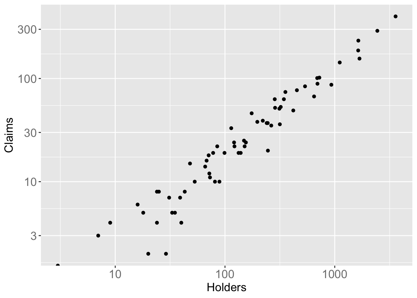
gg + scale_x_continuous(trans = "log") + scale_y_continuous(trans = "log")## Warning: Transformation introduced infinite values in continuous y-axis
gg = ggplot(data=mtcars)

gg + geom_density(aes(x=mpg))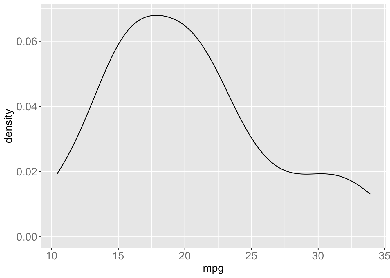
gg + geom_density(aes(x=mpg), size=1.2)
gg + geom_density(aes(x=mpg, color=factor(gear)), size=1.2)
gg + geom_density(aes(x=mpg, color=factor(gear), linetype=factor(gear)), size=1.2)
gg + geom_density(aes(x=mpg, color=factor(gear), linetype=factor(gear), fill=factor(gear)), size=1.2)
gg + geom_density(aes(x=mpg, color=factor(gear), linetype=factor(gear), fill=factor(gear)), size=1.2, alpha=0.2)
gg = ggplot(data=economics) + geom_path(aes(x=unemploy/pop, y=psavert), size=1.2)
gg
# "geom_hline" does the same thing as "geom_abline" with slope=0.
gg + geom_abline(intercept = mean(economics$psavert), slope = 0) + geom_vline(xintercept = mean(economics$unemploy/(economics$pop)))