Homework on unobserved heterogeneity
22 February, 2023
In this homework, we are going to consider a simple model of unobserved heterogeneity. We will do this through the lense of unemployment duration.
A simple model
We index individual by \(i\) and we suppose that we observe their unemployment spell. Each period the unemployed individual chooses how much effort to put into searching for work. This effort affects the probability \(\lambda_i\) of getting a job offer at wage \(W_i\). The cost to achieve arrival probability is given by \(c(\lambda_i)\). When he accecpts the job, we assume that the worker keeps the job for ever. The discount rate is \(r\) and we will consider \(r \rightarrow 0\).
The value of finding a job is given by \(V_e = \frac{\rho W}{r}\). Where \(\rho\) captures the tax system. The unemployed worker Bellman equation is then given by
\[ \begin{align} V_u & = \max_\lambda b - c(\lambda) + \lambda \frac{\rho W}{(1+r) r} + \frac{1-\lambda}{1+r} V_u \end{align} \] Question 1 show that for a fixed \(\lambda\) we can write:
\[ V_u = \frac{1+r}{r+\lambda} \Big( b - c(\lambda) + \lambda \frac{\rho W}{(1+r) r} \Big) \]
We are going to assume that \(c(\lambda) = \frac{a}{\gamma} \lambda^{(1+\gamma)}\).
Question 2 Show that taking the first order condition on the effort decision, and taking the limit \(r \rightarrow 0\), gives the following optimal choice for \(\lambda\):
\[ \lim_{r \rightarrow 0} \lambda = \Big( \frac{\rho W - b}{a}\Big)^{\frac{1}{1+\gamma}} \]
Simulating data
We draw wages from a log-nornmal distribution and attach the \(\lambda\) we derived previously.
set.seed(1234) # force the random state to get alwasys the same results

p = list(rho=0.9,a = 3, gamma =1.5)
p$n = 5000
data = data.table(B = 0, W = exp(rnorm(p$n) -3))

# solve for lambda
data[, Lb := ((p$rho*W - B)/(p$a))^(1/(1+p$gamma))]
data[, Lb := pmin(pmax(Lb,0),1)]

data[, D  := rexp(p$n, rate = Lb)]

ggplot(data,aes(x=W,y=Lb)) + geom_line() + theme_bw()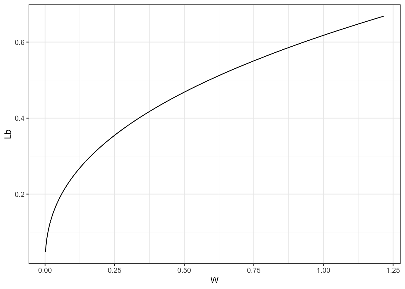
Estimating
In this first section we coinsider the simple case where all individuals are homogenous. We are interested in estimating \(a,\gamma\).
Question 3 Write down a function that computes the log-likelihood for a given data \(\{D_i,W_i\}_{i=1..N}\). Evaluate your log-likelihood $_i(a,) = _i [D_i|W_i;a,] $for a grid on \(a,\gamma\) around the truth and show that the max is around the true value.
Here is my likelihood function evaluated at the data simulated with the set random seed as well as second small data set for 3 points that you can use to check that you find the same values:
lik.homo(data$W,data$D,p)## [1] -13357.05lik.homo(c(0.014, 0.065, 0.147),c(19.2, 0.9, 9.7),p)## [1] -10.13286Here is what the answer should look like:
q1.plot()

We note that the MLE estimator of \(a\) for a given value of \(\gamma\) admits a close form solution.
Question 4 Derive the FOC condition for \(a\) from the likelihood expression, and find a close form solution for the solution.
Here is the value of my mle estimator for \(a\) evaluated at the true \(\gamma\):
mle.a(data$W,data$D,p$gamma,p$rho)## [1] 2.905502Random Effect
In this section we want to allow for individuals to have different values of \(a\). We assume that the population is devided in \(K\) groups, each having their own \(a_k\) parameter. We are going to only use \(K=3\).
Simulating data is as simple as before:
set.seed(1234) # force the random state to get alwasys the same results
p = list(rho=0.9,a = c(1,3,5), gamma =1.5, pk=c(0.2,0.5,0.3))

p$n = 1000
data = data.table(B = 0, W = exp(rnorm(p$n) -2))

# draw the latent type
data[, k := sample.int(3,.N,prob = p$pk,replace=T)]

# solve for lambda
data[, Lb := ((p$rho*W - B)/(p$a[k]))^(1/(1+p$gamma))]
data[, Lb := pmin(pmax(Lb,0),1)] # bound it between 0 and 1

data[, D := rexp(p$n, rate = Lb)]

head(data,5)
## B W k Lb D
## 1: 0 0.04047520 2 0.17128689 0.3488155
## 2: 0 0.17860640 2 0.31017537 4.9099833
## 3: 0 0.40029287 3 0.34918867 2.4318662
## 4: 0 0.01296246 3 0.08854907 6.8688337
## 5: 0 0.20786316 2 0.32957898 3.6596561Question 5 write down a function that computes the liklihood of the data given our random effect model. Show that this likelihood picks close to the true value of \(\gamma,a_1,a_2,a_3,p_1,p_2,p_3\) by varying each parameter separatly and reporting the likelihood (the \(p\) parameters need to sum to 1).
# your solution could look something like this
q2.plot()
Here, I would like for you to write the EM algorithm to recover the different types. We are going to write an Em to recover the \(a_k\) for a given \(\gamma\). Start with the true value of \(gamma\) for now. You need write code that:
- E-step: compute the posterior probability for each individual to be of type \(i\). ie \(q_i(k) = \text{Pr}[k_i = k | W_i ,D_i, \theta^\tau]\)
- M-step: code that computes the \(a_k\) parameters. You can use the close form you derived at the begining to do that.
Question 6 Write down a function that performs the EM estimation for a fixed value of \(\gamma\).
# for example my estep function gives the following on the first 5 rows of the data
d.estep = data.frame(em.estep(data$W[1:5],data$D[1:5],p))
d.estep$k = data$k[1:5]
d.estep
## X1 X2 X3 k
## 1 0.2866644 0.4772924 0.2360433 2
## 2 0.1398053 0.5219297 0.3382650 2
## 3 0.1798614 0.5148550 0.3052836 3
## 4 0.2084673 0.5069281 0.2846046 3
## 5 0.1652792 0.5180584 0.3166624 2# another way to check your code is to verify that when evaluated at the truth, the posterior probabilities aggregate to the prior
qik = em.estep(data$W,data$D,p)
colMeans(qik) # this should be the same as p$pk## [1] 0.1991835 0.4997466 0.3010699# finally I check that my M-step gives me close to the true value when evaluated at the truth
pnew = em.mstep(data$W,data$D,p,qik)
pnew$a## [1] 1.005750 3.117868 5.308934pnew$pk## [1] 0.1991835 0.4997466 0.3010699Within each EM step, the likelihood has to be going up, otherwise it means that you have an error. You can start from the true value here.
# finally, we can start at different value and loop
ptau    = copy(p)
#ptau$pk = c(0.3,0.3,0.4)
#ptau$a  = c(1,2.5,5)

rr = data.frame()
for (iter in 1:500) {
  qik  = em.estep(data$W,data$D,ptau)
  ptau = em.mstep(data$W,data$D,ptau,qik)
  Lik  = lik.hetero(data$W,data$D,ptau)
  rr = rbind(rr,data.frame(iter=iter,L=Lik))
}

ggplot(rr,aes(x=iter, y=L)) + geom_line() + geom_line() + theme_bw()
ptau## $rho
## [1] 0.9
##
## $a
## [1] 0.7594356 3.4033321 5.2080398
##
## $gamma
## [1] 1.5
##
## $pk
## [1] 0.2029926 0.4945379 0.3024696
##
## $n
## [1] 1000Question 7 wrap your EM algorithm in a grid over \(\gamma\). It should be reaching the highest value at the true \(\gamma\). You can start all parameters at the truth within each iteration.
q3.plot()
Fixed Effect
We could also have tried a fixed effect approach, where we directly use the duration as a measurement of the true lambda. In the Fixed Effect world, we estimate an \(a_i\) per individual. For a given individual you only have one \(D_i,W_i\). Still however, you can write the MLE estimate of \(a_i\) using the same formula that you derived at the begining of the homework.
We can try to maximize the overall likelihood using FE parameters \(a_i\) by applying the following procedure:
- for a given value of \(\gamma\) compute the MLE estimate of \(a_i\)
- evaluate the likelihood at the value of \(\gamma\)
- do this for a grid of \(\gamma\) and report what seems to be the highest value.
Question 8 Implement this in a function, report the estimate of \(\gamma\) that it returns (please actually report a curve over \(\gamma\)). Use the following code to generate data. Comment on the result.
p = list(rho=0.9, gamma =1.5)

p$n = 1000
data = data.table(B = 0, W = exp(rnorm(p$n) -2))

# draw the latent type
data[, a := runif(p$n, min=0.5, max=2.5)]

# solve for lambda
data[, Lb := ((p$rho*W - B)/a)^(1/(1+p$gamma))]
data[, Lb := pmin(pmax(Lb,0),1)] # bound it between 0 and 1

data[, D1 := rexp(p$n, rate = Lb)]
data[, D2 := rexp(p$n, rate = Lb)]
Question 9 (bonus) Repeat the fixed-effect approach for the case that we observe two sets of wage and unemployment duration. Specifically, we generate the data by the following code.
p = list(rho=0.9, gamma =1.5)

p$n = 1000
data = data.table(B = 0, W1 = exp(rnorm(p$n) -2), W2 = exp(rnorm(p$n) -2))

# draw the latent type
data[, a := runif(p$n, min=0.5, max=2.5)]

# solve for lambda
data[, Lb1 := ((p$rho*W1 - B)/a)^(1/(1+p$gamma))]
data[, Lb2 := ((p$rho*W2 - B)/a)^(1/(1+p$gamma))]
data[, Lb1 := pmin(pmax(Lb1,0),1)] # bound it between 0 and 1
data[, Lb2 := pmin(pmax(Lb2,0),1)] # bound it between 0 and 1

data[, D1 := rexp(p$n, rate = Lb1)]
data[, D2 := rexp(p$n, rate = Lb2)]